H₂ Formation

This test has a single reaction with a constant rate, which means there is an exact solution to compare against at every point in time, not only at the end. Because the chemistry is so simple, what it really exercises is the integrator rather than the network.

The network

File: networks/h2form/react_h2form.jet (PRIZMO format)

H + H -> H2   []   1e-17

There are two species: H and H2. The generated indices are idx_h and idx_h2.

What it checks

The rate coefficient is a constant, so nothing here depends on temperature, on an equation of state, or on any other species. What remains is the ODE on its own:

\[\frac{dn_{\text{H}}}{dt} = -2\,k\,n_{\text{H}}^2, \qquad \frac{dn_{\text{H}_2}}{dt} = +\,k\,n_{\text{H}}^2\]

which integrates exactly:

\[n_{\text{H}}(t) = \frac{n_{\text{H},0}}{1 + t/\tau}, \qquad \tau = \frac{1}{2\,k\,n_{\text{H},0}}, \qquad n_{\text{H}_2}(t) = \frac{n_{\text{H},0} - n_{\text{H}}(t)}{2}\]

Because the answer is known at every instant, you can measure the error directly rather than only spotting outright failure, and watch how that error responds as you tighten tolerances.

The factor of two

Both reactants are the same species, so each reaction event removes two H atoms. JAFF's generated right-hand side already accounts for this: the flux is k n_H², and it enters dn_H/dt twice. So if the measured τ comes out a factor of two off while the shape of the curve looks right, the most likely explanation is that the host code is applying its own duplicate-reactant convention on top of the one already in the generated code.

Setup

Quantity	Value	Note
Temperature	anything, e.g. `100 K`	The rate does not use it; set something valid for your EOS.
Initial `n_H`	`6.0e7 cm⁻³`	Gives `τ = 8.3333e8 s`.
Initial `n_H2`	`0`	Start fully atomic.
End time	`1e3 τ` (`8.33e11 s`)	Long enough that `n_H` has dropped three decades.
Output	log-spaced from `1e-4 τ`	The interesting error behaviour is early.

Density only rescales time

As with cie_h, the reaction is second order, so the solution depends on t and n_H0 only through the ratio t/τ. Any starting density works, as long as you rescale the end time to keep t/τ covering the same range.

What to plot

Left: n_H/n_H0 and 2 n_H2/n_H0 against t/τ, log-log, with the analytic curve overlaid. Right: the relative error of n_H against the analytic solution, same x-axis.

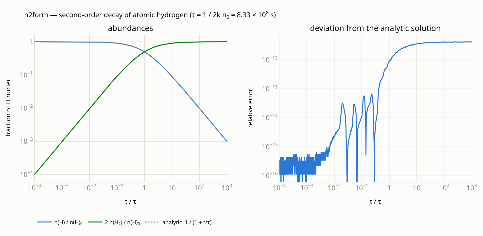
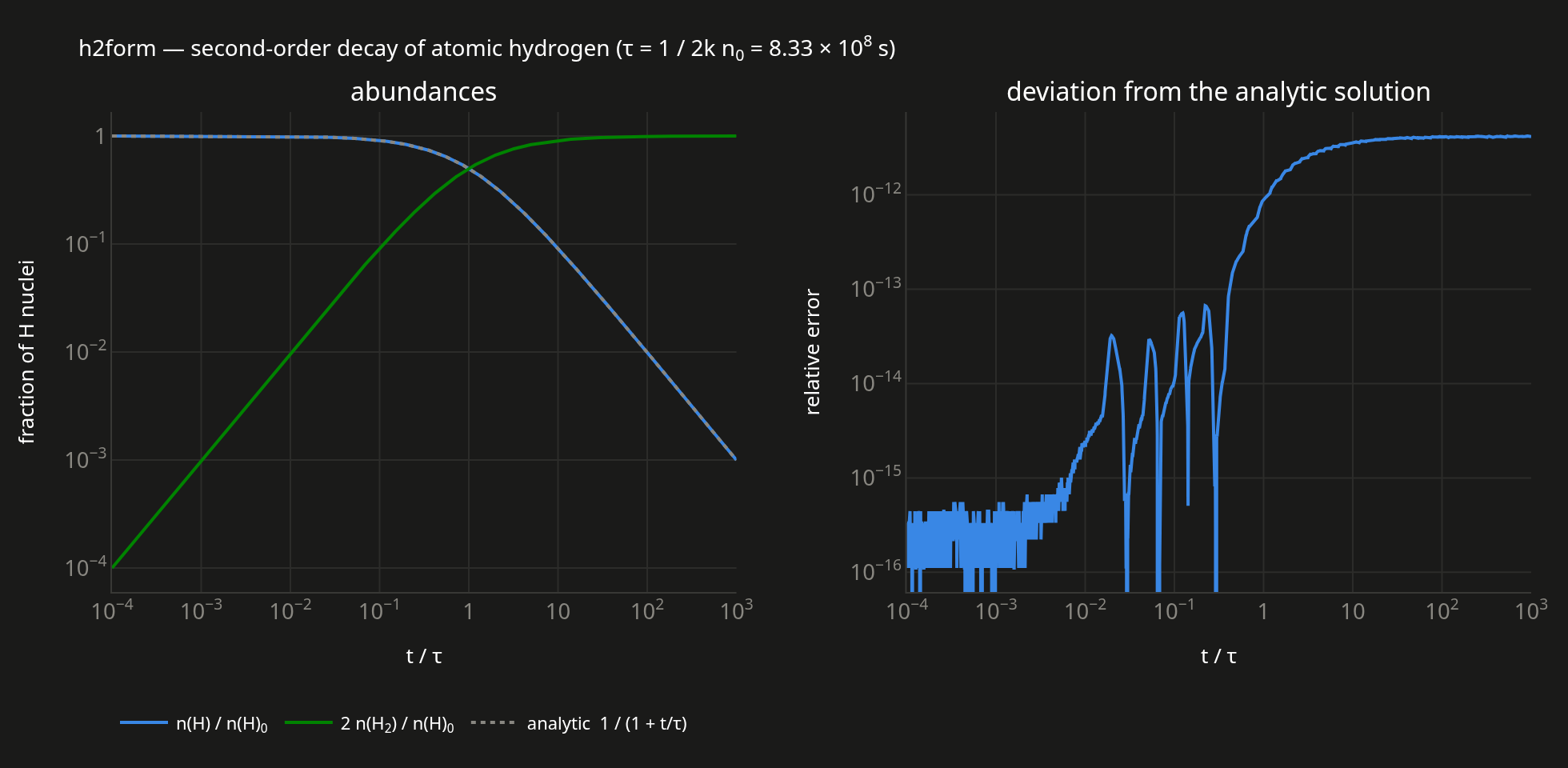
Atomic hydrogen decaying as 1/(1+t/tau) while H2 rises, with the relative error against the analytic solution staying below 1e-11

Two features of the left panel are worth reading off directly. The curves cross at t/τ = 1 by construction, and n_H becomes a straight line of slope −1 once t ≫ τ. A late-time slope that is not −1 points to the wrong reaction order — something a single end-state comparison would miss entirely.

The right panel shows what a reference-quality run looks like: error near round-off early on, growing to about 1e-11 as the steps accumulate. A production run will sit higher than this, and that is entirely expected.

What to expect

With n_H0 = 6.0e7 cm⁻³ and k = 1e-17 cm³ s⁻¹:

\[\tau = \frac{1}{2\,k\,n_{\text{H}^0}} = 8.3333 \times 10^{8}\,\text{s}\]

`t/τ`	`n_H/n_H0`	`2 n_H2/n_H0`
0.1	0.909091	0.090909
1	0.500000	0.500000
10	0.090909	0.909091
100	0.009901	0.990099
1000	0.000999	0.999001

Suggested acceptance:

Quantity	Threshold
largest relative error of `n_H` against the analytic	< 10 × your solver's `rtol`
largest departure of `(n_H + 2 n_H2) / n_H0` from 1	< 1e-10
fitted `τ` from the late-time slope	within 1% of `1 / (2 k n_H0)`

The first threshold is written in terms of your own tolerance on purpose: the point is whether the integrator delivers the accuracy it claims, not whether it hits some fixed number. A useful check is to halve rtol and see whether the error drops with it. If it does not, something other than truncation is setting the error floor — usually a species floor, a clip, or a wrong Jacobian.

Reference data

benchmarks/h2form/h2form_n6e7.txt — integrated at rtol = 1e-12, agreeing with the analytic solution to 4.2e-12 worst-case.

Column	Meaning
`t`	time (s), for `n_H0 = 6e7`
`t_tau`	`t / τ`
`n_H`	atomic hydrogen (cm⁻³)
`n_H2`	molecular hydrogen (cm⁻³)
`n_H_over_n0`	`n_H / n_H0`

Since the closed form is exact, you can skip the table entirely and compare against 1/(1 + t/τ) directly. The table is provided mainly to give a concrete sense of how close a well-converged run should get.

When it fails

Symptom	Cause
Curve has the right shape, `τ` off by exactly 2	Duplicate-reactant convention applied twice, or `k` interpreted as the per-atom rate.
Late-time slope is not −1	Reaction order wrong — the flux is not quadratic in `n_H`.
Error flat and large regardless of `rtol`	Jacobian wrong (the solver falls back to very small steps and its error estimate stops being meaningful), or a floor clamping `n_H2` early.
Error grows without bound after `t ≈ τ`	Explicit integrator, or step-size control disabled.
`n_H + 2 n_H2` drifts	Renormalization or clipping enabled; neither is appropriate here.
Early curve looks like straight segments	Output cadence too coarse. Sample logarithmically; the integrator is likely fine.