Worked Example

This page works through an example of how to use JAFF to auto-generate a chemistry network that can be integrated as part of an external hydro code. In this toy example, we will use a tiny network and a C++ template file that is self-contained rather than part of a larger hydro code, but that can still be compiled to produce a program that integrates the chemistry in time.

The layout mirrors the way things work in production. A real target code already owns its ODE-integration infrastructure — solvers, time-stepping, drivers — in its own files; JAFF only supplies a generated file holding the right-hand side (RHS) and Jacobian of the network along with other required properties. So the example is split across three files:

The mental model is the only thing to hold onto: a template is ordinary source code; every line is copied to the output verbatim except the $JAFF blocks, which are expanded against the network. The Template Syntax page is the full directive reference; this page just puts the pieces together.

1. The network

For this simple example, we will create a new, toy network, which consists of only two species and two reactions: hydrogen atoms forming H₂ and H₂ breaking back apart. Save it as toy.jet:

# Toy H2 formation/dissociation network (PRIZMO format)
# columns:  reaction  [tmin,tmax]  rate-coefficient(tgas)
H + H -> H2     []   1.00e-10*(tgas/3e2)**(-0.5)
H2 -> H + H     []   2.00e-9*exp(-1.0e2/tgas)

Both rates are plain functions of the gas temperature tgas, so the generated code is self-contained — no photochemistry, cosmic-ray, or extinction symbols to supply at runtime. Species are indexed in load order: H is 0, H2 is 1.

2. The template

The template produces only the network-specific code: the species/reaction counts, the ODE right-hand side, and the analytic Jacobian. There is no solver and no main here — those belong to the host code (sections 4 and 5). The output is a header the rest of the program #includes. Save it as chem_rhs.hpp. The $JAFF blocks are the only generated regions — everything else is C++ copied through untouched.

// chem_rhs.hpp — a JAFF template.
// Every line is plain C++ copied verbatim, except the $JAFF blocks, which JAFF
// fills in from the network. The output is a header the host code #includes.
#pragma once
#include <cmath>

// $JAFF SUB nspec, nreact
constexpr int NSPEC  = $nspec$;
constexpr int NREACT = $nreact$;
// $JAFF END

// dn/dt for every species. nden = number densities (cm^-3), tgas = K.
inline void derivatives(const double* nden, double tgas, double* f) {
    // $JAFF REPEAT idx, ode IN odes
    f[$idx$] = $ode$;
    // $JAFF END
}

// Analytic Jacobian J[i][j] = d f[i] / d nden[j]. Only the non-zero entries are
// generated; the rest stay zero from the clear loop.
inline void jacobian(const double* nden, double tgas, double** J) {
    for (int i = 0; i < NSPEC; ++i)
        for (int j = 0; j < NSPEC; ++j) J[i][j] = 0.0;
    // $JAFF REPEAT idx, expr IN jacobian
    J[$idx$][$idx$] = $expr$;
    // $JAFF END
}

Three directives carry the whole template:

• SUB nspec, nreact swaps the $nspec$ / $nreact$ tokens for the counts.
• REPEAT idx, ode IN odes emits one f[$idx$] = $ode$; line per species, filling $idx$ with the species index and $ode$ with the full dn/dt expression. The odes collection inlines the rate coefficients, so the rates never need a separate array here.
• REPEAT idx, expr IN jacobian emits the analytic Jacobian. It is a 2D collection, so the body carries two $idx$ tokens (row, then column) and one $expr$. JAFF differentiates the ODEs symbolically and writes only the non-zero J[i][j] entries — which is why the function clears J to zero first. The implicit solver in section 4 needs this matrix; an explicit method would not.

The Jacobian is written into a 2D array passed as double** J, indexed J[i][j]. The double-pointer form carries no compile-time size, so the integrator in section 4 can allocate J at runtime from the nspec it is given and stay completely network-independent — it never has to know NSPEC. The generated code uses NSPEC only as the loop bound when it clears J, since here it is the file that owns that constant.

The comment token (//) is read from the .hpp extension; JAFF recognises a directive only when a line begins with it immediately followed by $JAFF. The generated code uses the names nden and tgas, so the host code below speaks the same names — no remapping needed.

3. Generate

Run jaffgen over the template, pointing it at the network:

jaffgen --network toy.jet --files chem_rhs.hpp --outdir generated/

INFO     Network loaded successfully!
INFO     chem_rhs.hpp created at .../generated
INFO     Successfully generated files

The expanded file keeps its name and lands in generated/chem_rhs.hpp. The directive lines survive in the output (as comments), with the generated content spliced in beneath them:

// $JAFF SUB nspec, nreact
constexpr int NSPEC  = 2;
constexpr int NREACT = 2;
// $JAFF END

// dn/dt for every species. nden = number densities (cm^-3), tgas = K.
inline void derivatives(const double* nden, double tgas, double* f) {
    // $JAFF REPEAT idx, ode IN odes
    f[0] = -3.4641016151377544e-9*std::pow(tgas, -0.5)*std::pow(nden[0], 2) + 4.0000000000000002e-9*std::exp(-100.0/tgas)*nden[1];
    f[1] = 1.7320508075688772e-9*std::pow(tgas, -0.5)*std::pow(nden[0], 2) - 2.0000000000000001e-9*std::exp(-100.0/tgas)*nden[1];
    // $JAFF END
}

// Analytic Jacobian J[i][j] = d f[i] / d nden[j]. Only the non-zero entries are
// generated; the rest stay zero from the clear loop.
inline void jacobian(const double* nden, double tgas, double** J) {
    for (int i = 0; i < NSPEC; ++i)
        for (int j = 0; j < NSPEC; ++j) J[i][j] = 0.0;
    // $JAFF REPEAT idx, expr IN jacobian
    J[0][0] = -6.9282032302755089e-9*std::pow(tgas, -0.5)*nden[0];
    J[0][1] = 4.0000000000000002e-9*std::exp(-100.0/tgas);
    J[1][0] = 3.4641016151377544e-9*std::pow(tgas, -0.5)*nden[0];
    J[1][1] = -2.0000000000000001e-9*std::exp(-100.0/tgas);
    // $JAFF END
}

Each J[i][j] is the partial derivative of f[i] with respect to nden[j] — here all four entries are non-zero, but on a real network the Jacobian is sparse and JAFF emits only the entries that survive differentiation.

4. The integrator

The following solver is host-code infrastructure. In a real hydro code this is the existing ODE-integration layer that already lives in its own source files; here it is a small backward-Euler step. Save it as integrator.hpp.

The integrator is network-independent: it names no species, takes the species count nspec as a plain int argument, and works on double** matrices it allocates at runtime. It never includes the generated header — it only needs the RHS and Jacobian, which the driver hands it as function pointers. The same solver drives a two-species toy and a thousand-species network without recompilation.

// integrator.hpp — backward-Euler ODE integration infrastructure.
// Hand-written host code in its own file, the way a hydro code keeps its solver
// layer separate from the generated chemistry. It is network-independent: it
// names no species, takes the species count as an argument, and receives the
// RHS / Jacobian as function pointers.
#pragma once
#include <cmath>
#include <utility>
#include <vector>

// The RHS / Jacobian signatures the generated code provides.
using rhs_fn = void (*)(const double* nden, double tgas, double* f);
using jac_fn = void (*)(const double* nden, double tgas, double** J);

// Solve A x = b in place for an n-square system (Gaussian elimination with
// partial pivoting). A is a 2D matrix (A[i][j]) and n is passed in by the caller
// — the call shape a reusable solver layer exposes. b holds the solution.
inline void solve(int n, double** A, double* b) {
    for (int col = 0; col < n; ++col) {
        int piv = col;
        for (int r = col + 1; r < n; ++r)
            if (std::fabs(A[r][col]) > std::fabs(A[piv][col])) piv = r;
        for (int c = 0; c < n; ++c) std::swap(A[col][c], A[piv][c]);
        std::swap(b[col], b[piv]);
        for (int r = col + 1; r < n; ++r) {
            double m = A[r][col] / A[col][col];
            for (int c = col; c < n; ++c) A[r][c] -= m * A[col][c];
            b[r] -= m * b[col];
        }
    }
    for (int r = n - 1; r >= 0; --r) {
        double s = b[r];
        for (int c = r + 1; c < n; ++c) s -= A[r][c] * b[c];
        b[r] = s / A[r][r];
    }
}

// One implicit backward-Euler step of size dt: solve
// y_new - y - dt*f(y_new) = 0 for y_new by Newton iteration, where the Newton
// matrix is I - dt*J. nspec is supplied by the caller, not hardwired.
inline void backward_euler_step(int nspec, double* y, double tgas, double dt,
                                rhs_fn derivatives, jac_fn jacobian) {
    std::vector<double> yn(y, y + nspec), f(nspec), res(nspec);
    // Newton matrix G and Jacobian J as 2D arrays, exposed as double**.
    std::vector<std::vector<double>> Gstore(nspec, std::vector<double>(nspec));
    std::vector<std::vector<double>> Jstore(nspec, std::vector<double>(nspec));
    std::vector<double*> G(nspec), J(nspec);
    for (int i = 0; i < nspec; ++i) { G[i] = Gstore[i].data(); J[i] = Jstore[i].data(); }

    for (int it = 0; it < 8; ++it) {
        derivatives(yn.data(), tgas, f.data());
        jacobian(yn.data(), tgas, J.data());
        for (int i = 0; i < nspec; ++i) {
            res[i] = -(yn[i] - y[i] - dt * f[i]);
            for (int j = 0; j < nspec; ++j)
                G[i][j] = (i == j ? 1.0 : 0.0) - dt * J[i][j];
        }
        solve(nspec, G.data(), res.data());     // res <- Newton update
        double norm = 0.0;
        for (int i = 0; i < nspec; ++i) { yn[i] += res[i]; norm += std::fabs(res[i]); }
        if (norm < 1.0e-6) break;
    }
    for (int i = 0; i < nspec; ++i) y[i] = yn[i];
}

G and J are std::vector<double*> views over per-row storage, so passing G.data() / J.data() gives the double** the solver and the generated jacobian expect, and every access stays plain 2D A[i][j] indexing. The integrator receives the RHS and Jacobian as function pointers (rhs_fn / jac_fn), so it calls them through their signature rather than naming the network's chemistry directly.

5. The driver

Finally, the host driver wires the two halves together: it #includes the JAFF-generated header and the integrator, sets the initial conditions, and runs the time loop. Save it as main.cpp.

// main.cpp — the host driver: initial conditions, time loop, output.
// Hand-written host code. It includes the JAFF-generated RHS/Jacobian header and
// the integrator infrastructure, then wires the two together.
#include <cstdio>
#include "generated/chem_rhs.hpp"   // generated by JAFF: NSPEC, derivatives, jacobian
#include "integrator.hpp"           // host infrastructure: backward_euler_step

int main() {
    double nden[NSPEC] = {1.0e6, 0.0};   // start fully atomic: H, H2
    const double tgas = 3.0e2;           // 300 K
    const double dt   = 1.0e3;           // s
    const int    nsteps = 200;

    printf("%10s %12s %12s %14s\n", "t[s]", "n(H)", "n(H2)", "H_nuclei");
    for (int s = 0; s <= nsteps; ++s) {
        if (s % 40 == 0)
            printf("%10.0f %12.4e %12.4e %14.6e\n",
                   s*dt, nden[0], nden[1], nden[0] + 2*nden[1]);
        backward_euler_step(NSPEC, nden, tgas, dt, derivatives, jacobian);
    }
    return 0;
}

NSPEC, derivatives, and jacobian come from the generated header; the loop and backward_euler_step come from the host. Re-running jaffgen after a network change regenerates generated/chem_rhs.hpp in place and leaves integrator.hpp and main.cpp untouched.

6. Compile and run

Compile the driver — it pulls in both headers — and run it:

g++ -O2 -std=c++17 main.cpp -o toy_solver
./toy_solver

      t[s]         n(H)        n(H2)       H_nuclei
         0   1.0000e+06   0.0000e+00   1.000000e+06
     40000   1.1649e+05   4.4175e+05   1.000000e+06
     80000   6.0802e+04   4.6960e+05   1.000000e+06
    120000   4.1075e+04   4.7946e+05   1.000000e+06
    160000   3.1012e+04   4.8449e+05   1.000000e+06
    200000   2.4920e+04   4.8754e+05   1.000000e+06

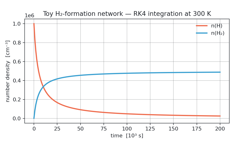
The atomic hydrogen converts to H₂ and settles toward chemical equilibrium, and the last column — total H nuclei, n(H) + 2·n(H2) — stays pinned at 1.0e6, the conservation check that says the integrator and the generated right-hand side agree. Plotting every step makes the approach to equilibrium plain:

This split is the whole point of the workflow. The chemistry stays in the network file, the solver infrastructure stays in your repo, and a single jaffgen command keeps the generated RHS and Jacobian in sync with the network — without ever editing the host code by hand.

See also

• Template Syntax — every directive, collection, and modifier.
• jaffgen CLI — inputs, built-in templates, and options.
• Codegen — the low-level generator behind the odes/rates/jacobian collections.
• Builder — ready-made solver templates when you don't want to write your own.