GOW Equilibrium
The first two tests compare JAFF against closed-form solutions. This one is different: there is no formula to check against, so instead it compares the generated network against an independent implementation — the equilibrium state of the Gong, Ostriker & Wolfire (2017) network, computed with a separate code and reproduced here.
The network
Files: networks/GOW/GOW.jet, GOW.jfunc, GOW.hdf5 — the network in KIDA format, its custom rate and heating/cooling functions, and the interpolation tables those functions read. See Predefined Networks for what each file contains.
It has eighteen species and about fifty reactions, and — unlike the other two tests — the gas temperature is part of what gets solved rather than something you hold fixed.
What it checks
The parts of the pipeline the two small tests do not touch:
- auxiliary functions — rate coefficients defined in
.jfuncrather than as closed-form expressions (Auxiliary Functions); - table interpolation — cooling functions that read grids out of
GOW.hdf5, and their derivatives in the Jacobian (Table Interpolation); - thermal coupling — chemistry and temperature solved together, each feeding the other;
- environment parameters — the radiation field, extinction, cosmic-ray rate, metallicity and dust-to-gas ratio reaching the rates correctly.
A network this size has no analytic solution, but it is still testable because its equilibrium state traces out a curve. The idea is to hold everything fixed except the density, integrate to steady state at each density in turn, and check that the resulting sequence of states follows the reference.
Backend requirements
This test asks more of a host code than the other two. The backend needs to support HDF5 table interpolation, integrate a gas-energy equation alongside the species, carry number densities, and make the environment parameters below available at runtime.
The python_solve_ivp template does not meet these requirements — it generates the species equations only, and the GOW rate expressions refer to runtime state it does not provide. For this test you will need a backend that also solves a thermal equation, or you can wire the generated right-hand side into a driver of your own (see the worked example).
Setup
Environment
| Parameter | Value | Meaning |
|---|---|---|
chi |
0.1, 1, or 10 |
FUV radiation field strength, Draine units |
Av |
0 |
Visual extinction — unshielded gas |
| cosmic-ray rate | 2e-16 |
Primary ionization rate per H, s⁻¹ |
| metallicity | 1 |
Solar |
| dust-to-gas ratio | 0.01 |
Solar |
| redshift | 0 |
No CMB contribution |
Reference tables are provided for all three radiation fields on a shared density grid. Running chi = 10 on its own already exercises the network; running all three adds a check that the field strength reaches the photorates with the right scaling, which a single value cannot show on its own.
Initial state
Start at a temperature of 100 K, with the abundances below given relative to hydrogen. Multiply each by the total hydrogen density n_H of the run to recover number densities in cm⁻³:
| Species | x_i |
Species | x_i |
Species | x_i |
|---|---|---|---|---|---|
H |
1.0 | He |
1e-1 | C |
1e-40 |
H+ |
1e-4 | He+ |
1.45e-8 | C+ |
1.6e-4 |
e- |
3e-4 | O |
3.2e-4 | CO |
1.0e-7 |
H2 |
1e-10 | O+ |
1e-40 | HCO+ |
1e-40 |
H2+ |
1e-40 | OH |
1e-40 | CH |
1e-40 |
H3+ |
2.681411e-07 | Si |
1.7e-6 | Si+ |
1e-40 |
The initial state should not matter
These are the values used for the runs shown on this page, but keep in mind that the test measures a steady state. Perturbing the initial abundances should leave the endpoint unchanged; if it moves, either the integration is not running long enough, or a species has been driven to a value it cannot recover from (one pinned at exactly zero will stay there).
The 1e-40 entries stand for "absent", written that way so that logarithms and divisions stay well-defined. Only replace them with exact zeros if your host code is happy handling them.
The scan
Repeat the run at a series of densities, holding everything else fixed:
| Quantity | Value |
|---|---|
n_H |
10 → 981 cm⁻³, at least ~15 points spread logarithmically |
| density | constant during each run — no collapse, no free-fall |
| end time | 7e20 s |
| output | log-spaced; only the final state is compared |
The reference grid has 95 points spaced by a factor of 1.05, which is finer than the test needs — feel free to pick a subset, or use your own spacing and interpolate.
The end time is far longer than anything physical, and that is deliberate: it guarantees the endpoint is the steady state and not a snapshot part way there. A good way to confirm you have reached it is to check that the last decade of the integration changes nothing.
What to plot
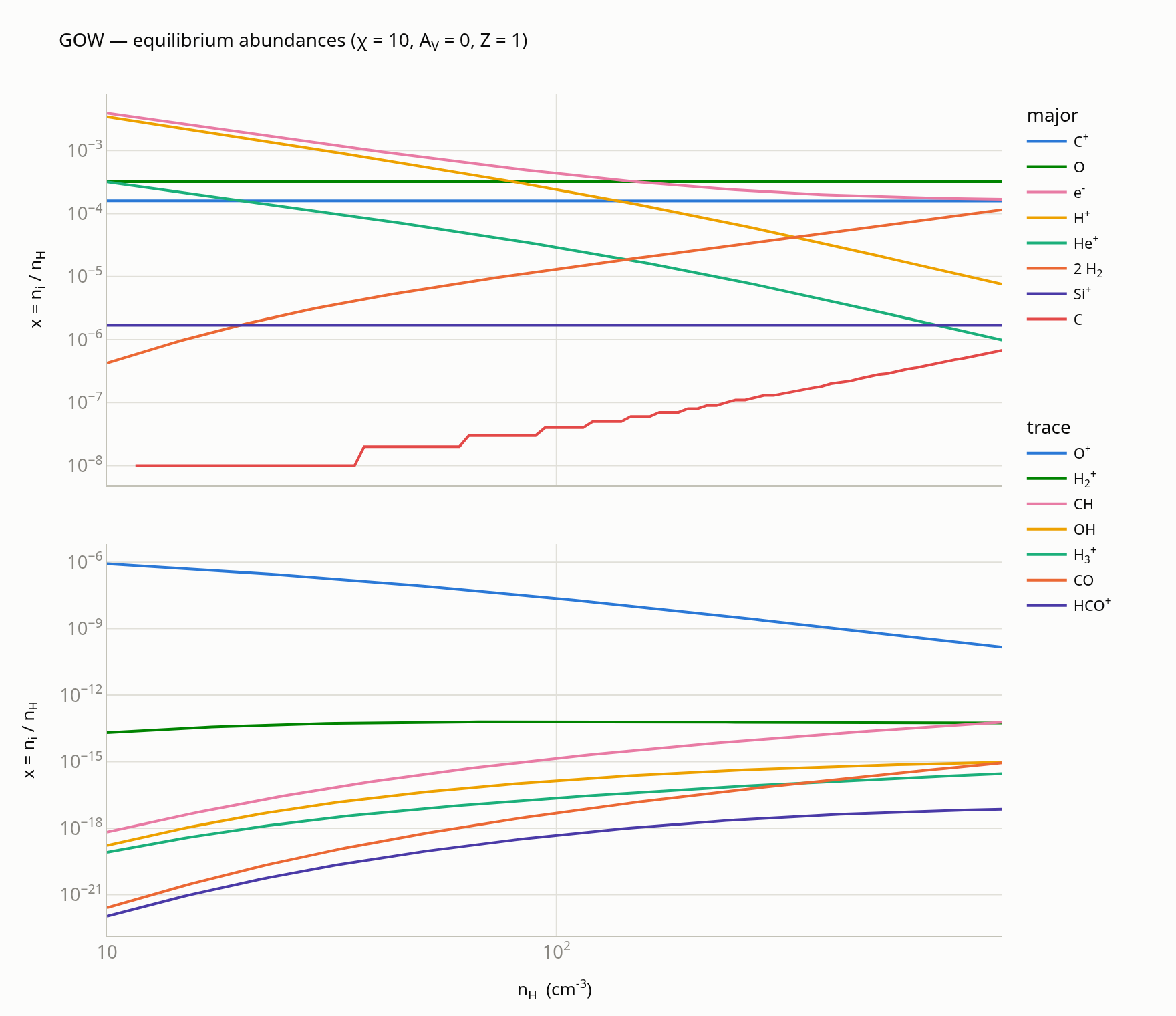
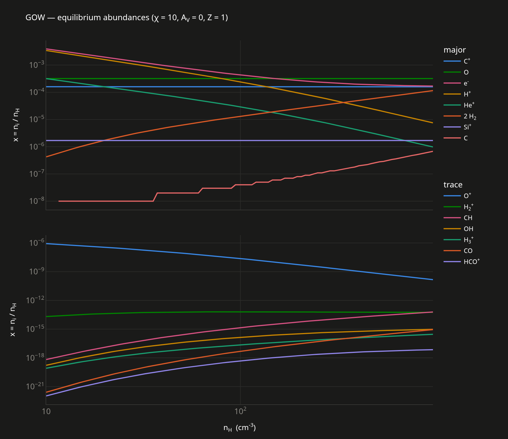
Plot the final abundances against n_H on log-log axes, and put the gas temperature on a separate plot rather than a second y-axis. The species span roughly twenty decades, so it helps to split them: the ones above 1e-7 are what the comparison really rests on, and the rest are useful mainly as a diagnostic. The figures below show the reference tables — a natural way to compare is to overlay your own final states as markers on the same axes.
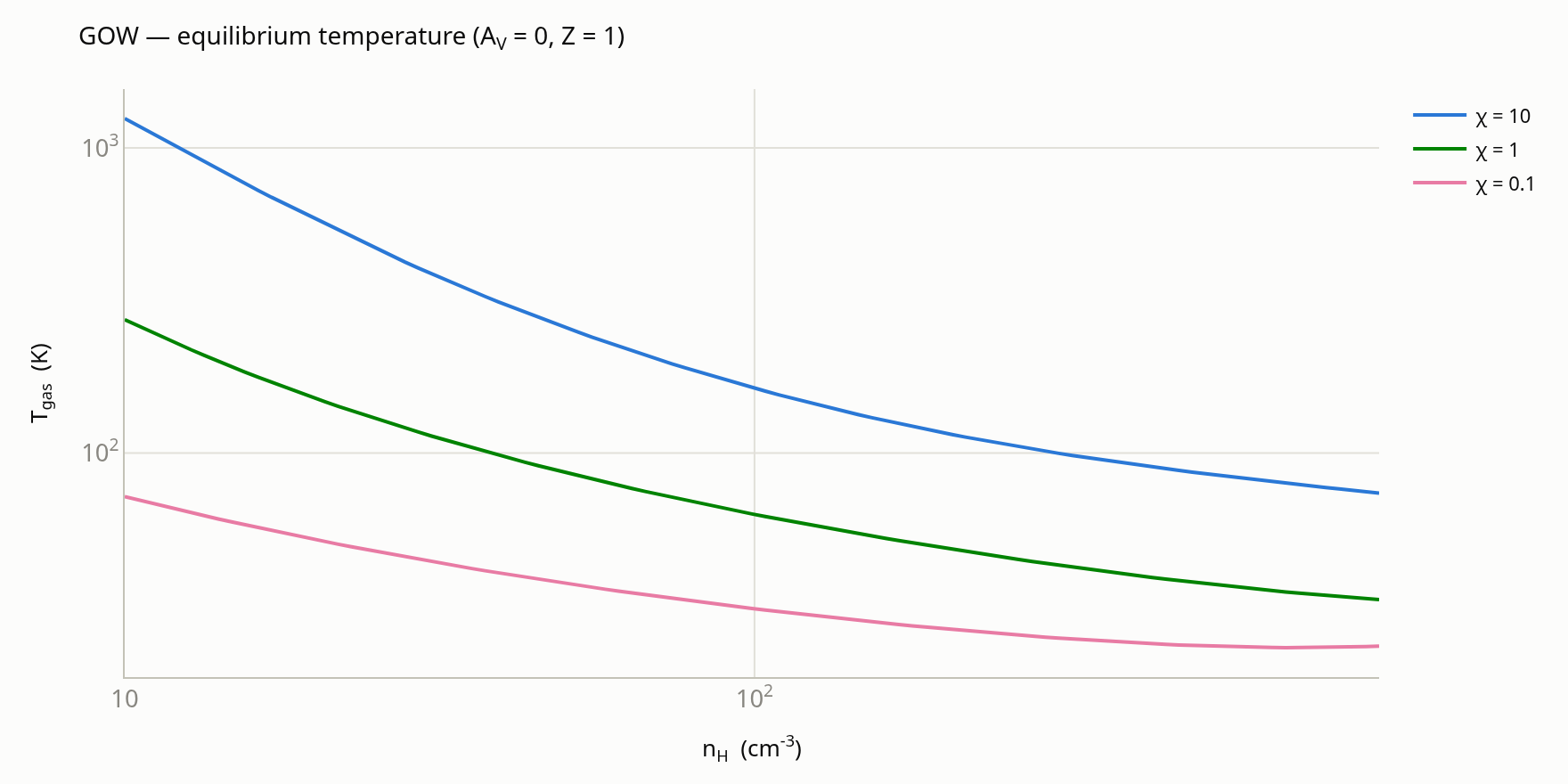
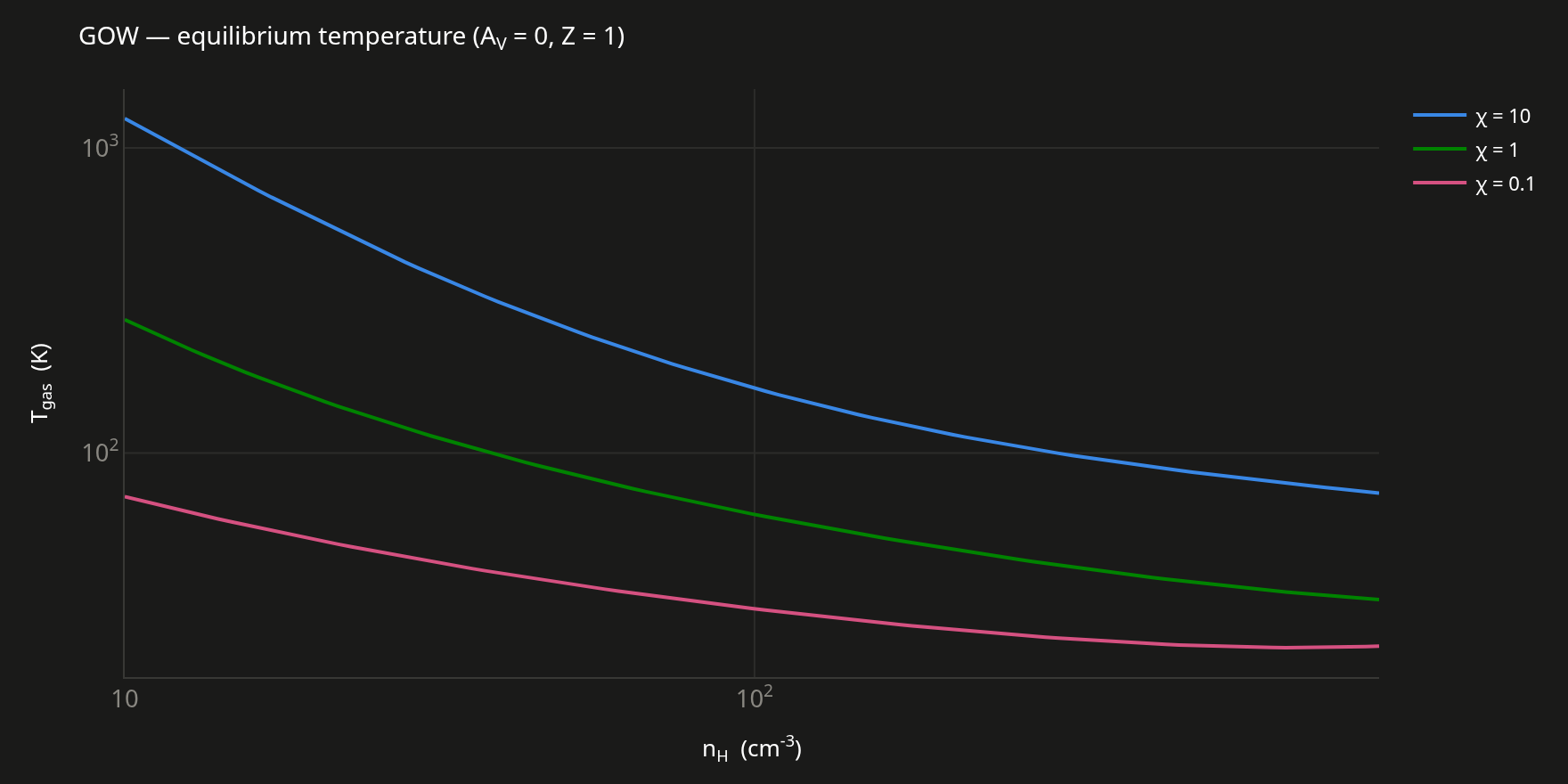
Temperature falls with density in all three radiation fields, offset roughly by the field strength:
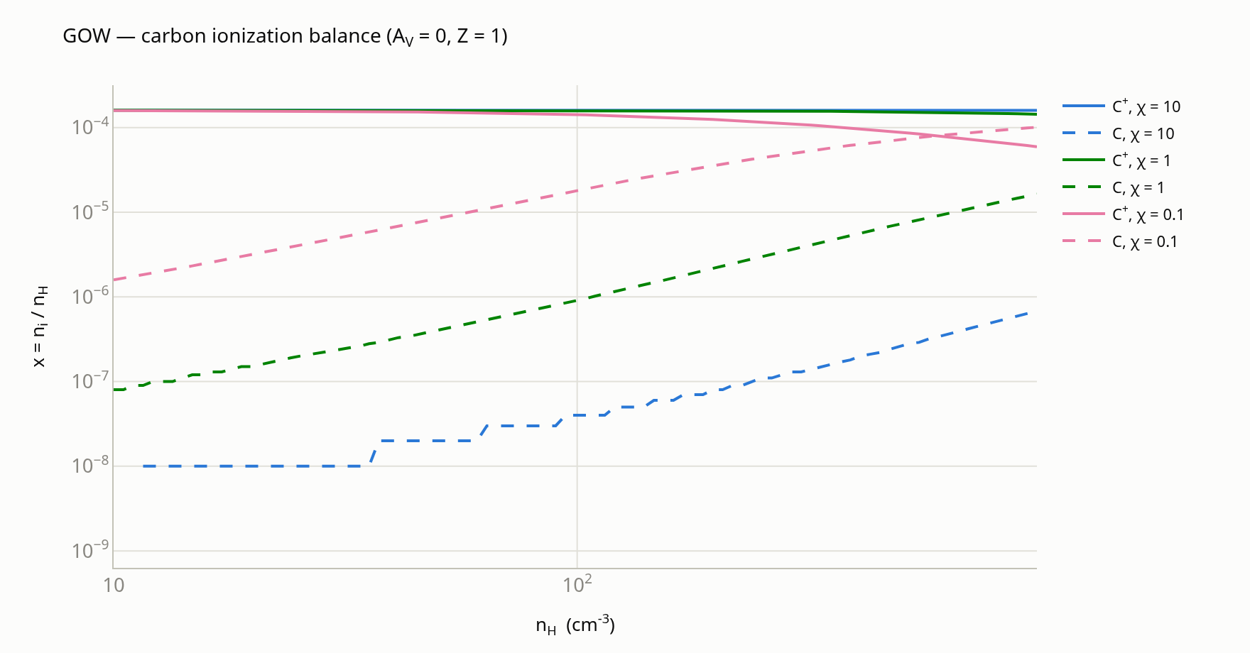
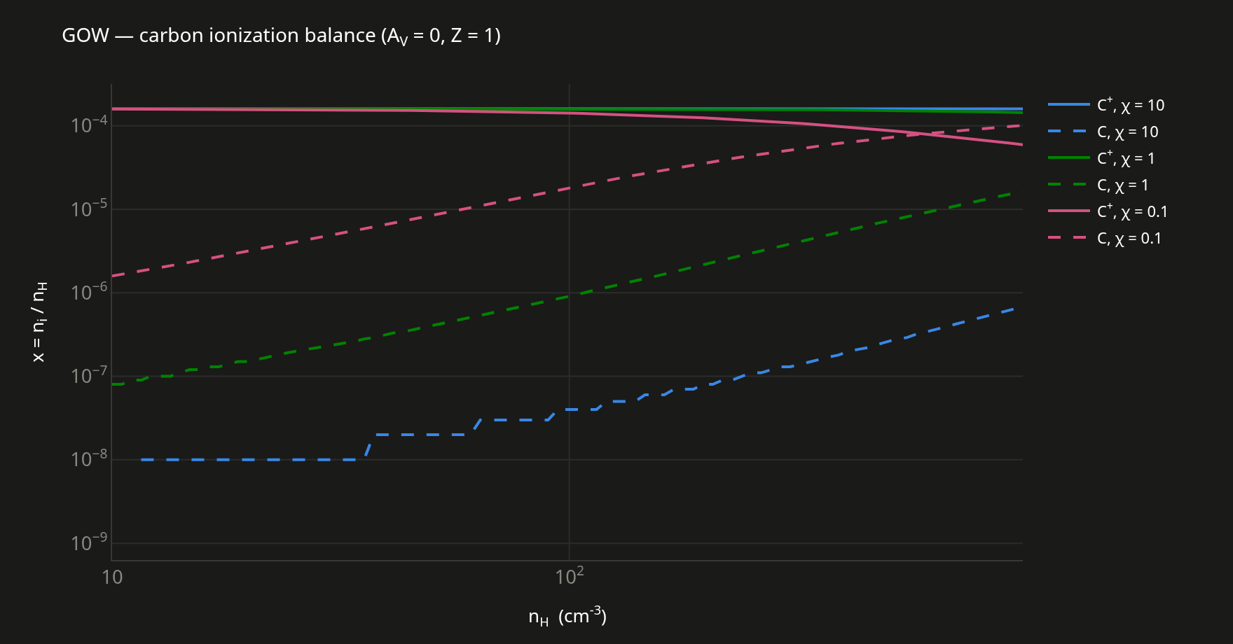
The carbon balance is the clearest way to tell the fields apart. At chi = 0.1, neutral carbon overtakes C⁺ near n_H ≈ 600 cm⁻³; at chi = 1 it climbs to about a tenth of C⁺ by the top of the range; and at chi = 10 it stays at least two decades below throughout:
Normalize by hydrogen, not by everything
The reference abundances are x_i = n_i / n_H, where n_H counts hydrogen nuclei: n(H) + n(H+) + 2 n(H2) + 2 n(H2+) + 3 n(H3+). If you divide by the total number density instead, helium gets folded in and every abundance shifts by about 10% — enough to look like a real disagreement when it is only a normalization mismatch.
What to expect
With Av = 0 the gas is unshielded at every field strength, so CO never builds up to anything significant — the highest CO abundance anywhere in the three tables is only 6e-12. What does change with density is the hydrogen and carbon ionization structure, along with the temperature.
At chi = 10, between the ends of the density grid:
| Quantity | at n_H = 10 cm⁻³ |
at n_H = 981 cm⁻³ |
Behaviour |
|---|---|---|---|
T_gas |
1249.0 K | 73.9 K | falls monotonically, no plateau |
x(e-) |
3.930e-3 | 1.695e-4 | tracks H⁺ at low n, C⁺ at high n |
x(H+) |
3.451e-3 | 7.535e-6 | falls steeply |
x(He+) |
3.177e-4 | 9.824e-7 | falls steeply |
2 x(H2) |
4.260e-7 | 1.156e-4 | the only major species that rises |
x(C+) |
1.6000e-4 | 1.5932e-4 | essentially constant |
x(O) |
3.2000e-4 | 3.2000e-4 | constant — oxygen stays neutral |
x(Si+) |
1.7000e-6 | 1.6997e-6 | constant — silicon stays ionized |
By the high-density end, the electron abundance has fallen to roughly the carbon abundance: most of the protons and He⁺ have recombined, which leaves C⁺ as the main carrier of charge.
The same quantities across the three fields, at the two ends of the grid:
| Quantity | chi = 0.1 |
chi = 1 |
chi = 10 |
|---|---|---|---|
T_gas |
72.0 → 23.2 K | 273.6 → 33.0 K | 1249.0 → 73.9 K |
x(e-) |
5.895e-4 → 6.392e-5 | 1.410e-3 → 1.487e-4 | 3.930e-3 → 1.695e-4 |
x(H+) |
3.793e-4 → 2.578e-6 | 1.119e-3 → 2.931e-6 | 3.451e-3 → 7.535e-6 |
2 x(H2) |
1.171e-4 → 7.944e-3 | 1.239e-5 → 9.093e-4 | 4.260e-7 → 1.156e-4 |
x(C+) |
1.584e-4 → 5.932e-5 | 1.599e-4 → 1.436e-4 | 1.600e-4 → 1.593e-4 |
x(C) |
1.590e-6 → 1.007e-4 | 8.000e-8 → 1.635e-5 | ~0 → 6.800e-7 |
A weaker field means colder gas, more H₂, and more neutral carbon, and the trend is monotonic across all three. If your run reproduces chi = 10 but not the ordering between the fields, that usually means the field strength is reaching some photorates but not others.
Suggested acceptance, per density point:
| Quantity | Threshold |
|---|---|
T_gas |
within 5% |
species with x > 1e-7 |
within 10% |
species with x < 1e-13 |
within a factor of a few |
x(C+) + x(C) + x(CO) + x(HCO+) |
equals the carbon abundance, 1.6e-4, to 1e-6 relative |
The band on the trace species is wide for a reason. Down at x ~ 1e-20 the reference itself carries noise from its own solver, and small differences in how the cooling tables are interpolated push those numbers around without any physical meaning. The carbon sum is a different kind of statement: it follows from the structure of the network, and it holds to better than 1e-7 relative in all three reference tables, so it should hold just as tightly for any integrator.
Oxygen does not sum the same way
In the reference, x(O) sits at the full oxygen abundance 3.2e-4 at every density, while x(O+) is tracked on top of that. The oxygen-bearing species therefore sum to 3.2e-4 + x(O+) — up to 0.3% above the elemental total at the low-density end where O⁺ peaks. This is how the network was published rather than an error in the reference, so use carbon for the conservation check.
Reference data
benchmarks/GOW/equilibrium_chi0.1.txt, equilibrium_chi1.txt and equilibrium_chi10.txt — 95 rows each, with n_H running from 10 to 981.28 cm⁻³ in steps of a factor 1.05. They come from Munan Gong's PDR code with the parameters of Gong, Ostriker & Wolfire (2017). Since the three share a single density grid, they line up row by row. Rather than matching the reference spacing, interpolate the reference onto whatever grid your own run uses.
| Column | Meaning |
|---|---|
nH |
total hydrogen nuclei (cm⁻³) |
Tgas |
equilibrium gas temperature (K) |
2H2 |
2 x(H2) — the fraction of H nuclei locked in H₂ |
Cp, Hp, Hep, Sip, Op, H2p, H3p, HCOp |
ionized species, p for + |
C, O, CO, OH, CH, e |
neutral species and electrons |
There are two quirks of the files to be aware of before comparing. First, the 2H2 column is twice the H₂ abundance, not the abundance itself. Second, a few entries for very rare species carry slightly negative values (of order 1e-18, all in the chi = 10 table); these are numerical noise from the reference solver, so it is safe to treat anything below about 1e-17 as zero.
When it fails
| Symptom | Cause |
|---|---|
| Every abundance off by ~10%, shape correct | Normalizing by total number density instead of hydrogen nuclei. |
| H₂ column off by exactly 2 | The reference 2H2 column read as x(H2). |
| Temperature right, abundances wrong (or the reverse) | Chemistry and thermal balance not coupled — one is being solved at the other's fixed state. |
Trace species pinned at their initial 1e-40 |
Floor too high, or species clipping enabled. |
| Temperature settles far too high | A cooling channel returning zero: check that the GOW.hdf5 tables load and the interpolation is in range. |
| Endpoint depends on the initial state | Not integrated to steady state, or a species has been driven to exactly zero and cannot recover. |
Curve matches at low n_H, diverges at high n_H |
Dust-related terms (photoelectric heating, grain recombination) — check the dust-to-gas ratio and grain charge. |